ELECTRONIC COOLING IN CST STUDIO SUITE

Conjugate Heat Transfer (CHT) Solver

CST Studio Suite offers a dedicated Conjugate Heat Transfer (CHT) Solver to address your PCB thermal analysis along with other thermal applications like filters, antennas, etc. The Conjugate Heat Transfer solver is designed to simulate and analyze the heat transfer and fluid flow in typical electronics cooling applications, which usually involve all three modes of heat transfer using the Computational Fluid Dynamics (CFD) technique. The CHT solver uses octree-based cartesian meshing, which can be very tolerant of geometric issues often accompanying complex CAD geometries.

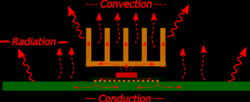
Figure 1. Heat Transfer Modes in a typical electronics application

Simulation Setup and workflow

CST supports ECAD imports of various formats which efficiently helps you set up your thermal simulations since all the necessary data is made available within a single user interface (e.g., M-CAD/E-CAD models, PCB layout with its stack-up and schematics, PCB component shapes, etc). The user can then run an IR-Drop analysis once the integrity of the E-CAD import is validated. IR-Drop analysis helps you understand the complexity of your model by analyzing the power loss distribution in your design and helps you identify the areas with major losses. Depending on if the power losses are prominent in the PCB layers compared to the components, you can then choose to use the whole PCB or a simplified geometry of the same.

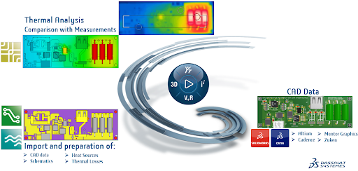
Figure 2. Workflow Overview

The EDA import window (Figure 3) can be used to control various import settings like components, Stackup layers, nets along with other PCB simplification options. The simplified model uses equivalent thermal properties and helps reduce the simulation time by reducing the model complexities.

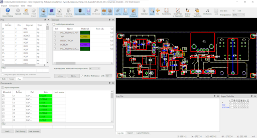
Figure 3. EDA Import Settings

Heat sources can be defined for the components through a single window (Figure 4) with the help of various import formats (e.g., csv, xml, etc). This avoids the inconvenience caused by manually selecting each component for entering their power ratings and helps save valuable time.

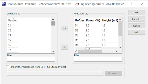
Figure 4. Heat Source definition

Once the E-CAD model is prepped, the user can then go about defining the various CFD conditions and parameters such as the boundary conditions, fluid domain, Nonlinear fan curve (for forced convection), vents and lids, etc and mesh the model.

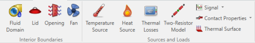
Figure 5. CFD boundaries and sources

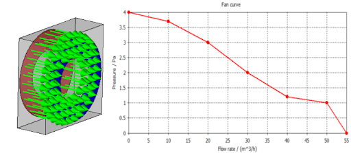
Figure 6. Fan definition with fan curve

The CFD mesh can be defined globally (background mesh) and locally (local refinement). Mesh control points can be used wherever necessary when certain boundaries need to be meshed (Figure 7). CHT solver parameters with respect to initial conditions, fluid flow, turbulence, radiation, simulation type (steady state/transient), goals, etc can be defined in the CHT solver window (Figure 8).

Figure 7. CFD Mesh with local refinement

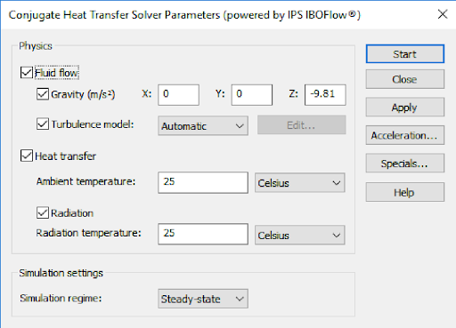
Figure 8 Solver settings

Post Processing features help visualize all calculated and monitored results like temperature generation, pressure, velocity vectors and heat flux in your model among many other results.

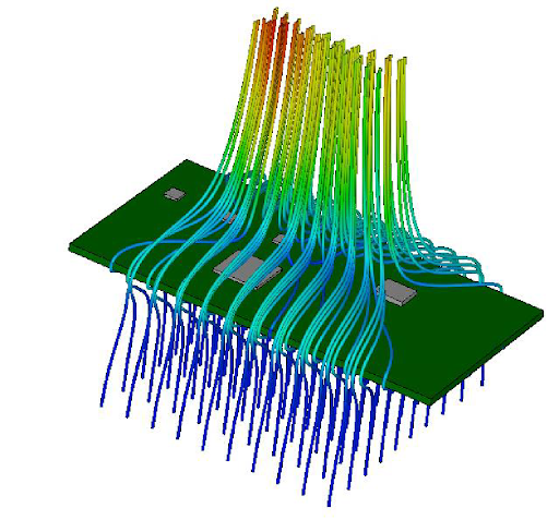
Figure 9 Flow streamlines

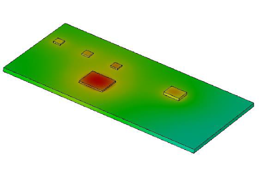
Figure 10 Temperature plot

Thus, CST Studio Suite also helps you address thermal challenges in your electronic modules efficiently along with other analyses like Signal/Power integrity, IR loss computation, EMC/EMI, shielding problems and much more within a single user interface.

We Urge You To Call Us For Any Doubts & Clarifications That You May Have. We Are Eager to Talk To You

Call Us: +91 7406663589